
 USA
USA Belgium
 France
 UK
UK Australia
 India
India Singapore
Table of Contents
1
Introduction
2
Overview
3
Quibit and Quantum State
4
Quantum Gates
5
Algorithms
6
Design & Testing
7
Conclusion
8
References
9
Glossary
10
Contributors
INTRODUCTION
Introduction

OVERVIEW OF QUANTUM MACHINE LEARNING
OVERVIEW OF QUANTUM MACHINE LEARNING
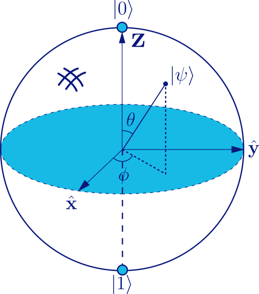
QUIBIT AND QUANTUM STATE
QUIBIT AND QUANTUM STATE

- |ψ+⟩=|00⟩ + |11⟩/ Ö2
- |ψ–⟩=|00⟩ – |11⟩/ Ö2
- |ψ+⟩=|01⟩ + |10⟩/ Ö2
- |ψ–⟩=|01⟩ – |10⟩/ Ö2

QUANTUM GATES
QUANTUM GATES
- A computer developed totally of billiard balls and mirrors, provides a beautiful concrete realization of the principles of reversible computation, and;
- A technique based on the Toffoli gate (a reversible logic gate), which can perform any computation that a classical computer can.

- Pauli-X: ….. It maps |0⟩ to |1⟩ and |1⟩ to |0⟩. It is equivalent to a NOT gate.
- Pauli-Y: ….. It maps |0⟩ to i |1⟩ and |1⟩ to −i |0⟩.
- Pauli-Z: ….. Also called a phase-flip, it leaves the basis state |0⟩ unchanged and maps |1⟩ to −|1⟩.
- Hadamard: H ….. It creates a superposition by mapping |0⟩ to and |1⟩ to .
- Phase shift: ….. It leaves the basis state |0⟩ unchanged and maps |1⟩ to eiψ |1⟩.
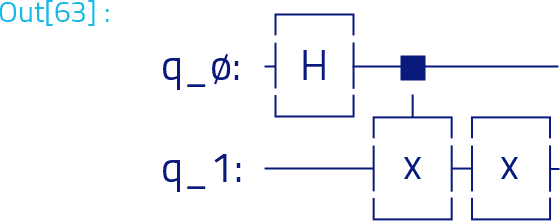
- Controlled NOT: …. It acts on 2 qubits and performs the NOT operation on the target qubit only when the control qubit is |1⟩.
- SWAP: …. It acts on 2 qubits and swaps these two qubits.
ALGORITHMS
ALGORITHMS
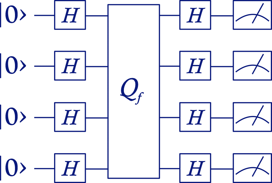
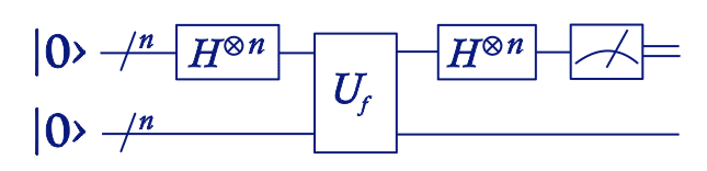
- |0⟩⊗n|1⟩ Initialize state.
- Create superposition using Hadamard gates.
- Calculate function f using Uf.
- Perform Hadamard transform
- Measure to obtain final output z.
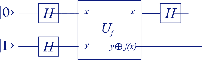
- Initialize state to the state, and output qubit to |−⟩.
- Apply Hadamard gates to the input register.
- Apply Hadamard gates to the output register.
- → 0 if si =0 and 1 if si=1 Measure to obtain final output s.
- y=y.z mod 2
- z=(x⊕s).z mod 2
- z=x.z⊕s.z mod 2
- 0=s.z mod 2
- Performed on classical computers: The classical part reduces the factorization to a problem of finding the period of the function.
- Performed on quantum machines: The quantum part uses a quantum computer to find the period using the Quantum Fourier Transform (QFT).
- If n is even, prime, or a prime power, then exit.
- Pick a random integer x < n and compute gcd (x, n). If it is not 1, then we have achieved a factor of n.
- Quantum algorithm: Pick q as the smallest power of 2 with n2 ≤ q < 2n2 . Find period r of xa mod n. The measurement gives us a variable c, which has the property c/q≈d/r where d ∈ N, where q is the dimension of a Hilbert space.
- To find d, r via continued fraction expansion algorithm. d and r are only determined if gcd(d, r) = 1 (reduced fraction).
- If r is odd, go back to 2. If x^(r/2)≡ −1 mod n, go back to 2. Otherwise, the factors p, q = gcd( x^(r/2)± 1, n).

DESIGN & TESTING
DESIGN & TESTING

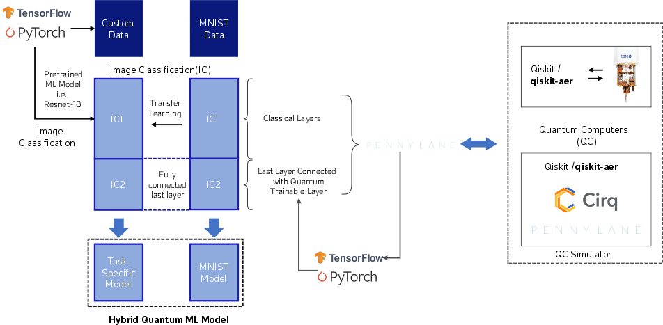 Figure 11. The architecture for the development of the hybrid quantum-classical ML
For study purposes, we are utilizing PyTorch integration with the Qiskit-Aer simulator using PennyLane to build our classification model. In this development, we are utilizing the hybrid-classical neural network approach, which is used for the development of a classification task with a pre-trained neural network architecture (ResNet-18) for classifying the images. Additionally, there are various connectors available, such as Pennylane, which can help to connect the PyTorch/TensorFlow conveniently to multiple quantum simulators and real quantum computers at the backend.
As shown in Figure 12, we have developed a quantum circuit for a multi-class hybrid classical model, which utilizes 6 qubits for the multiclass classification.
Figure 11. The architecture for the development of the hybrid quantum-classical ML
For study purposes, we are utilizing PyTorch integration with the Qiskit-Aer simulator using PennyLane to build our classification model. In this development, we are utilizing the hybrid-classical neural network approach, which is used for the development of a classification task with a pre-trained neural network architecture (ResNet-18) for classifying the images. Additionally, there are various connectors available, such as Pennylane, which can help to connect the PyTorch/TensorFlow conveniently to multiple quantum simulators and real quantum computers at the backend.
As shown in Figure 12, we have developed a quantum circuit for a multi-class hybrid classical model, which utilizes 6 qubits for the multiclass classification.
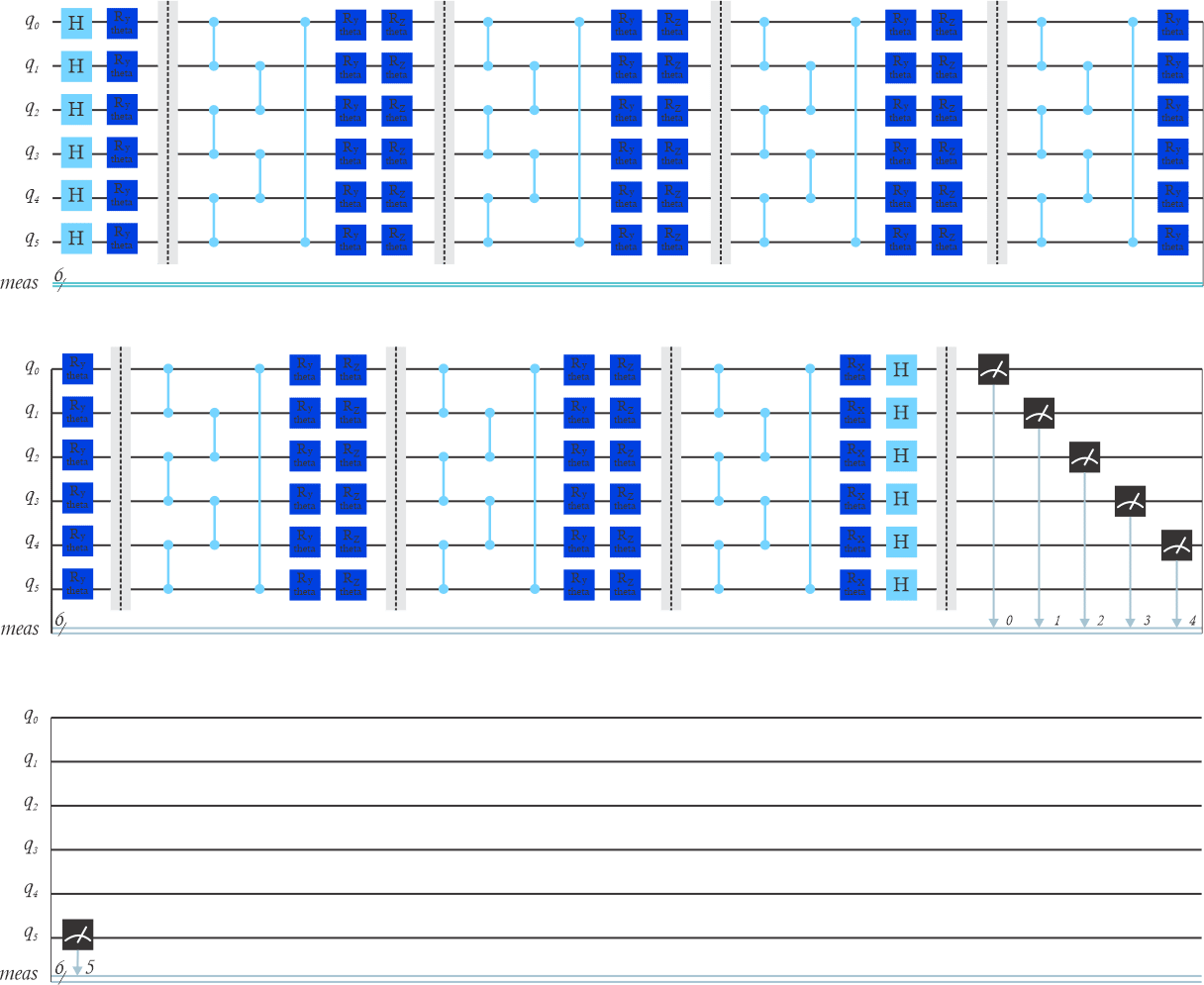 Figure 12. The quantum circuit for hybrid quantum-classical neural networks (HQCNN) for multi-class image classification
At the initial level, the 6-qubits are introduced to the Hamdard(H) gate to bring them to their superposition states. As the data embedding layer that takes inputs from the previous layer of the neural network, the output states from the H gate are processed with the Rotational Y (Ry) gate.
Figure 12. The quantum circuit for hybrid quantum-classical neural networks (HQCNN) for multi-class image classification
At the initial level, the 6-qubits are introduced to the Hamdard(H) gate to bring them to their superposition states. As the data embedding layer that takes inputs from the previous layer of the neural network, the output states from the H gate are processed with the Rotational Y (Ry) gate.
 Figure 13.
The entanglement layer created using Controlled Z(Cz) gate
The parametrized quantum circuit utilizes the Controlled Z(Cz) gate as an entanglement layer combined with Rotational Y (Ry) and Rotational Z (Rz) gate, which is repeated 6 times. The output from the last entanglement layer is rotated using the Rotational X(Rx) along with the H gate, and the result is measured in the Z-basis state from the quantum layer. To maintain the symmetry between the classical and quantum models’ hyperparameters, we have utilized the cross-entropy loss function with Adam optimizer and a learning rate of 0.001 and 0.0004.
We have tested the above quantum circuit on two different datasets: brain tumor and corrosion. We have created a custom brain tumor dataset containing 4500+ images to develop a multi-class brain tumor classification model. We have utilized transfer learning to replace the last layer for the resnet-18 with a quantum layer, which is then re-trained on the local quantum simulators for the development of the brain tumor model.
Table 1. Hyper-parameter values used for the classification model on different image datasets
Figure 13.
The entanglement layer created using Controlled Z(Cz) gate
The parametrized quantum circuit utilizes the Controlled Z(Cz) gate as an entanglement layer combined with Rotational Y (Ry) and Rotational Z (Rz) gate, which is repeated 6 times. The output from the last entanglement layer is rotated using the Rotational X(Rx) along with the H gate, and the result is measured in the Z-basis state from the quantum layer. To maintain the symmetry between the classical and quantum models’ hyperparameters, we have utilized the cross-entropy loss function with Adam optimizer and a learning rate of 0.001 and 0.0004.
We have tested the above quantum circuit on two different datasets: brain tumor and corrosion. We have created a custom brain tumor dataset containing 4500+ images to develop a multi-class brain tumor classification model. We have utilized transfer learning to replace the last layer for the resnet-18 with a quantum layer, which is then re-trained on the local quantum simulators for the development of the brain tumor model.
Table 1. Hyper-parameter values used for the classification model on different image datasets
| Parameters | Metal Corrosion | Brain Tumor |
| Quantum Depth | 31 | 31 |
| Number of Epochs | 100 | 200 |
| Batch Size | 8 | 16 |
| Learning Rate | 0.0004 | 0.001 |
| Max Accuracy Achieved During Iterations | 100% | 96.62% |
| Dataset | Metal Corrosion |
| Best Accuracy | 100% |
| Test Results | 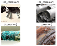 |
| Accuracy Results | 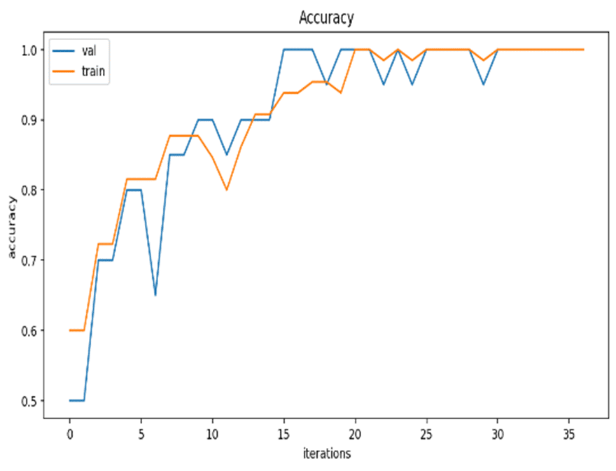 |
| Loss Results | 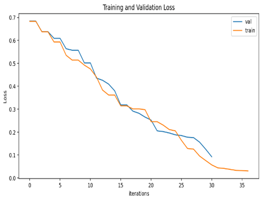 |
| Evaluation Metrics | 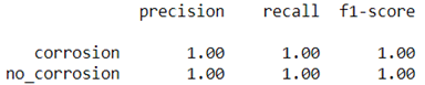 |
| Dataset | Brain Tumor (Multi-class) |
| Best Accuracy | 96.62% |
| Test Results | 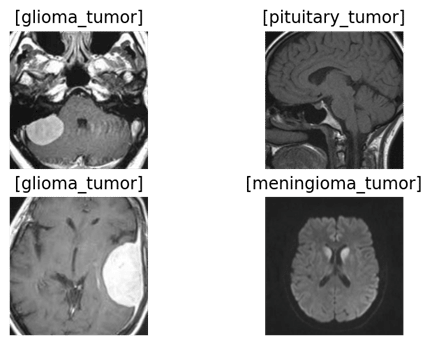 |
| Accuracy Results | 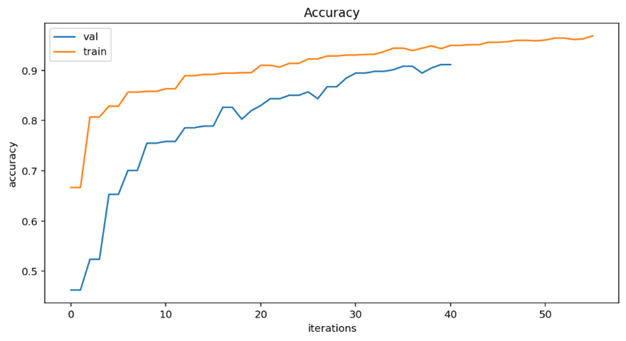 |
| Loss Results | 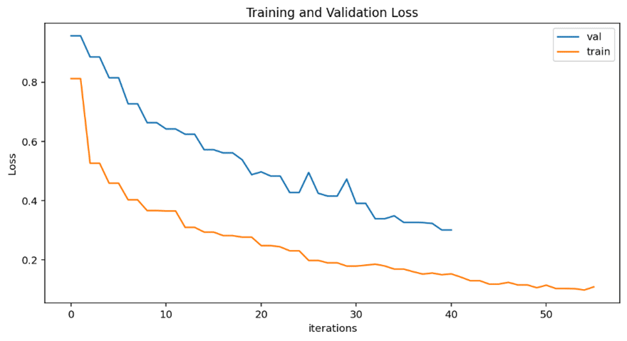 |
| Evaluation Metrics | 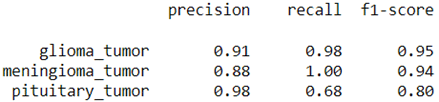 |
CONCLUSION
CONCLUSION

REFERENCES
REFERENCES

- Menard, Alexandre, et al. “A game plan for quantum computing.” McKinsey Quarterly, February 6, 2020.
- Sandhu, Adarsh. “Quantum Computing: Technology with limitless possibilities looking for tough problems to solve.” Springer Nature, 2018.
- Adcock, Jeremy, et al. “Advances in quantum machine learning.” Quantum Engineering Centre for Doctoral Training, University of Bristol, December 10, 2015.
- TA-Swiss. Quantum Technologies, 2021
- Yanofsky, Noson S., and Mirco A. Mannucci. Quantum Computing for Computer Scientists. Cambridge University Press, August 2008.
- Tensorflow Quantum Computing, 2021. www.tensorflow.org
- José D. Martín-Guerrero, Lucas Lamata. “Quantum Machine Learning: A tutorial”, Neurocomputing, 2021.
- QuIC Seminar. “The Bernstein-Vazirani Algorithm.” Michigan State University.
- Watrous, John. “Lecture 6: Simon’s algorithm.” University of Waterloo, February 2, 2006.
- Grant Salton, Daniel Simon, and Cedric Lin. Exploring Simon’s Algorithm with Daniel Simon, 2021
- Erdi ACAR and Ihsan YILMAZ. COVID-19 detection on IBM quantum computer, 2020
- Junhua Liu,1, 2 Kwan Hui Lim. Hybrid Quantum-Classical Convolutional Neural Networks, 2021. arxiv.org
- Peter Young. The Bernstein-Vazirani Algorithm, 2019
- Chih-Chieh Chen, Shiue-Yuan Shiau, Ming-Feng Wu & Yuh-Renn Wu. Hybrid classical-quantum linear solver using Noisy Intermediate-Scale Quantum machines, 2019
- Andrea Mari, Thomas R. Bromley, Josh Izaac, Maria Schuld, Nathan Killoran. Transfer learning in hybrid classical-quantum neural networks, 2020
- Ville Bergholm, Josh Izaac, Maria Schuld, Christian Gogolin. PennyLane: Automatic differentiation of hybrid quantum-classical computations, 2020
- IBM Qiskit textbook. qiskit.org
- Changyu Dong. Math in Network Security
- Elisa Baumer, Jan-Grimo Sobez, Stefan Tessarini. Shor’s Algorithm, 2015
- Marcello Benedetti, Erika Lloyd, Stefan Sack, Mattia Fiorentini. Parameterized quantum circuits as machine learning models, 2019
- Post-Quantum Cryptography, NIST
- Carlos Bravo-Prieto, Ryan LaRose, M. Cerezo, Yigit Subasi, Lukasz Cincio, Patrick J. Coles. Variational Quantum Linear Solver, 2019
- Andi Sama. Hello Tomorrow,I am a Hybrid Quantum Machine Learning, 2020
- Aidan Pellow-Jarman. Near Term Algorithms for Linear Systems of Equations, 2021
- Aidan Pellow-Jarman, Ilya Sinayskiy. A Comparison of Various Classical Optimizers for a Variational Quantum Linear Solver, 2021
- Isaac Chuang and Michael Nielsen. Quantum Computation and Quantum Information, 2010
- QuIC Seminar. The Bernstein-Vazirani Algorithm
GLOSSARY
GLOSSARY
| |0⟩ | Qubit state with vector output (1, 0) |
| |1⟩ | Qubit state with vector output (0,1) |
| σx, σy and σz | Pauli sigma matrices |
| ⊕ | Modulo two additions |
| U | Unitary operator or matrix |
| H | Hadamard gate |
| α, β, γ, and δ | Real-valued number |
| |ψ⟩ | Superpositions |
| |+⟩ | Positive state phase |
| |-⟩ | Negative state phase |
| θ and ψ | Point on the unit’s three-dimensional sphere |
| |ψ+⟩ | Positive phase state |
| |ψ–⟩ | Negative phase state |
| ⊗ | Tensor product |
| I | Identity Matrix |
| H⊗n | Parallel action of n Hadamard gates |
| Rx | Rotational X gate |
| Ry | Rotational Y gate |
| Rz | Rotational Z gate |
| † | Hermitian conjugate |
Contributors

Arvind Ramachandra
Vice President of Technology & Cloud Services

Munish Singh
Deputy Manager, Research & Advisory AI/ML
About Innova Solutions
Innova Solutions is a leading global information technology services and consulting organization with 30,000+ employees and has been serving businesses across industries since 1998. A trusted partner to both mid-market and Fortune 500 clients globally, Innova Solutions has been instrumental in each of their unique digital transformation journeys. Our extensive industry-specific expertise and passion for innovation have helped clients envision, build, scale, and run their businesses more efficiently.
We have a proven track record of developing large and complex software and technology solutions for Fortune 500 clients across industries such as Retail, Healthcare & Lifesciences, Manufacturing, Financial Services, Telecom and more. We enable our customers to achieve a digital competitive advantage through flexible and global delivery models, agile methodologies, and battle-proven frameworks. Headquartered in Duluth, GA, and with several locations across North and South America, Europe and the Asia-Pacific regions, Innova Solutions specializes in 360-degree digital transformation and IT consulting services.
For more information, please reach us at – [email protected]